In the vast landscape of machine learning, few architectures have captured the imagination and transformed the field as profoundly as the Transformer. Like a master anatomist approaching a complex organism, we must carefully dissect each component to understand how this remarkable architecture breathes life into modern AI systems.
Since its introduction in the groundbreaking 2017 paper Attention is All You Need, the Transformer has become the backbone of revolutionary models like GPT, BERT, and countless others that now power everything from chatbots to code generators. What makes this architecture so special isn’t just its performance, it’s the elegant way it processes information, abandoning the sequential constraints that limited previous models and instead embracing a more holistic, attention-driven approach.
Grab your scalpel and prepare to explore the intricate organs that compose this revolutionary architecture. Each component plays a vital role, orchestrating a symphony of mathematical transformations that have redefined our understanding of sequence modeling and beyond.
By the end of our anatomical journey, you’ll understand not just what each part does, but why the Transformer’s design was such a leap forward in artificial intelligence.
The Evolutionary Context: Why Transformers Emerged#
Before cutting it open, let’s understand the evolutionary pressures that birthed the Transformer architecture.
Traditional recurrent networks (RNNs) processed sequences like a reader parsing text word by word, carrying forward a hidden state, a kind of computational memory that accumulated information as it moved through the sequence. But this sequential processing created significant bottlenecks, much like trying to understand a symphony by listening to one note at a time while forgetting the melodies that came before.
This design imposed harsh limitations: RNNs not only struggled with long sequences due to their inability to maintain coherent long-term dependencies, but they also made training painfully slow and unstable because of the Vanishing Gradient problem. Gradients would either explode or fade to nothing as they propagated backward through time, making it nearly impossible for the network to learn meaningful patterns across extended sequences.
The Transformer emerged in 2017 with a radical proposition: Attention is All You Need. This wasn’t merely a technical advancement: it represented a philosophical shift in how we conceptualize information processing. Instead of sequential digestion, the Transformer enables parallel comprehension, allowing the model to perceive entire sequences simultaneously and weigh the importance of each element in relation to all others. It’s like viewing a painting in its entirety rather than tracing its brushstrokes one by one, capturing both fine details and the broader compositional relationships that give the work its meaning.
The Skeletal Framework: Architecture Overview#
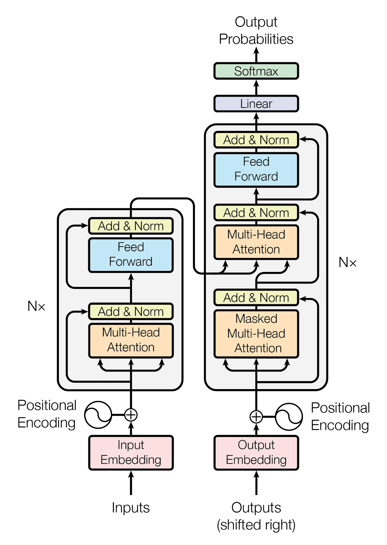
The Transformer’s anatomy consists of two primary sections: the encoder and the decoder. Think of them as the sensory and motor systems of our computational organism: the encoder ingests and comprehends input sequences, while the decoder generates responses based on this understanding.
The encoder stack processes the input sequence in its entirety, building rich representations that capture both the meaning of individual elements and their relationships to one another. Meanwhile, the decoder stack takes these representations and generates output sequences one token at a time, but with the crucial ability to attend to all previously generated tokens and the full encoded input simultaneously.
This dual-stack architecture enables the Transformer to excel at sequence-to-sequence tasks like translation, summarization, and question answering. However, it’s worth noting that many modern applications use only one half of this system: encoder-only models like BERT for understanding tasks, or decoder-only models like GPT for generation tasks.
But before any processing begins, we must address a fundamental challenge that seems almost paradoxical: how does a parallel architecture understand sequence order? After all, if we’re processing everything simultaneously, how does the model know that “The cat sat on the mat” is different from “Mat the on sat cat the”? Enter our first vital organ.
The Positional Encoding: The Transformer’s Spatial Awareness#
Imagine trying to understand a sentence with all words presented simultaneously, but without knowing their order. This is the challenge facing our Transformer: since the architecture processes the entire sequence in parallel, it inherently loses the spatial information about where each token sits in the sequence.
Positional encoding serves as the architecture’s proprioceptive system, its sense of where things are in space and time. Without this crucial component, the Transformer would be like a reader with perfect comprehension but no ability to distinguish between “The dog bit the man” and “The man bit the dog.”
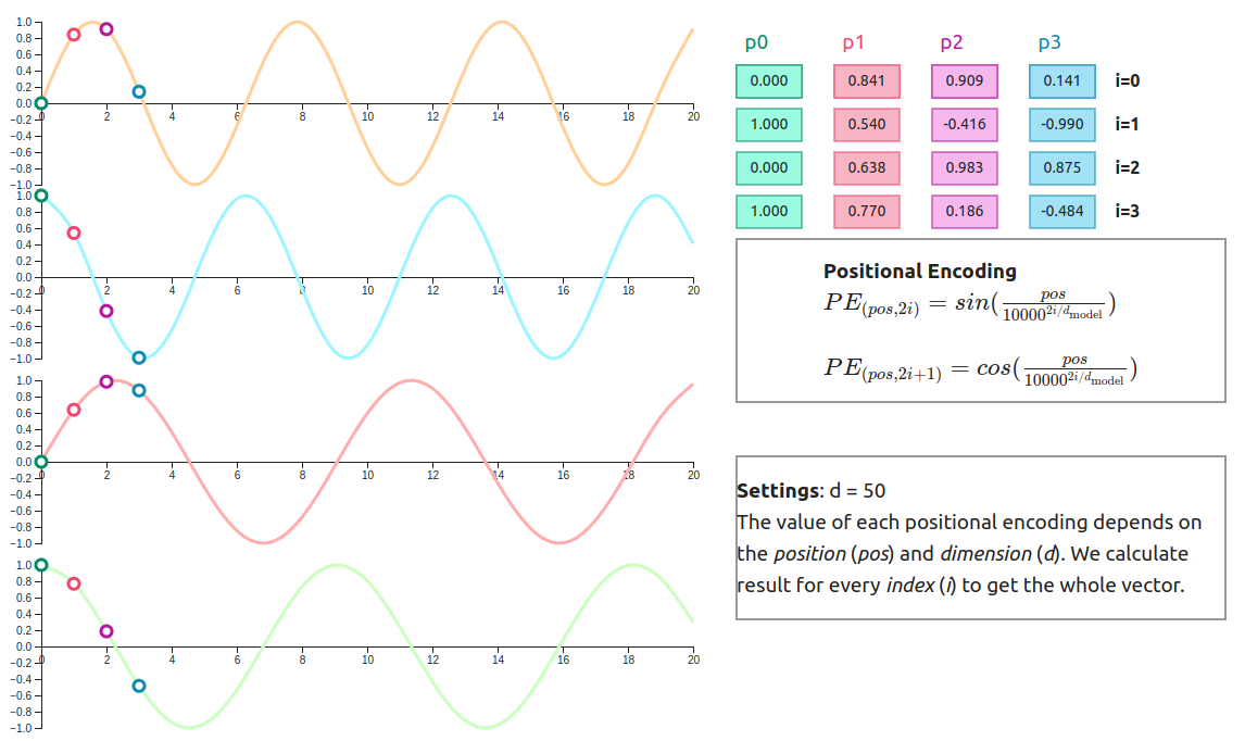
The mathematical elegance of positional encoding lies in its use of sinusoidal functions:
PE(pos, 2i) = sin(pos / 10000^(2i/d_model))
PE(pos, 2i+1) = cos(pos / 10000^(2i/d_model))
Where pos is the position in the sequence, i is the dimension index, and d_model is the model’s embedding dimension.
These functions create unique positional fingerprints that the model can learn to interpret. The genius lies in using different frequencies across dimensions, creating a rich positional vocabulary that’s both learnable and generalizable. Low frequencies capture broad positional patterns (distinguishing between the beginning, middle, and end of sequences), while high frequencies encode fine-grained distinctions between adjacent positions. This multi-scale approach mirrors how our visual system processes information, using different spatial frequencies to capture both coarse shapes and intricate details.
The sinusoidal choice isn’t arbitrary: it allows the model to potentially extrapolate to sequence lengths longer than those seen during training, since the mathematical relationships between positions remain consistent regardless of absolute sequence length.
But knowing where each word sits is only half the battle. The real magic happens when the Transformer decides what to pay attention to.
The Attention Mechanism: The Heart of the Transformer#
If positional encoding provides spatial awareness, attention represents the Transformer’s consciousness, its ability to focus on relevant information while maintaining awareness of the entire context. This mechanism embodies a profound insight: understanding emerges not from isolated analysis but from the dynamic interplay of relationships between all elements in a sequence.
Consider how you read this sentence right now. Your brain doesn’t process each word in isolation. Instead, it’s constantly relating “you,” “read,” “this,” and “sentence” to build meaning. The Transformer’s attention mechanism replicates this cognitive process computationally, allowing every position to simultaneously consider its relationship with every other position.
The Mathematics of Attention#
At its core, attention computes a weighted sum of values based on the compatibility between queries and keys:
Attention(Q, K, V) = softmax(QK^T / √d_k)V
But this formula, elegant as it is, barely hints at the profound computational process it represents. Let’s unpack each component:
- Queries (Q): These represent what each position is “asking for”, the information it needs to better understand its role in the sequence.
- Keys (K): These advertise what information each position contains, like labels on filing cabinets announcing their contents.
- Values (V): The actual information content to be retrieved and aggregated, like the files inside those cabinets.
The dot product between queries and keys measures compatibility, how relevant each piece of information is to each position’s needs. A high dot product means “this key answers this query well.” The scaling factor (√d_k) prevents the dot products from growing too large in high-dimensional spaces, maintaining stable gradients during training and ensuring the softmax doesn’t become too peaked.
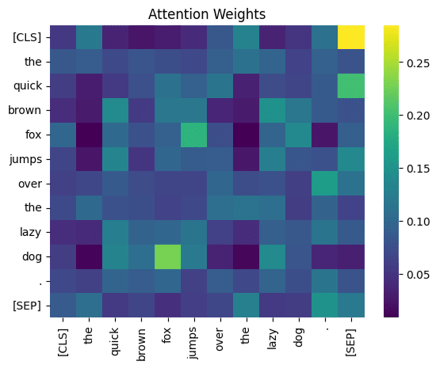
Self-Attention: The Introspective Mechanism#
Self-attention allows the model to relate different positions within the same sequence. It’s literally the sequence paying attention to itself. When processing “The cat sat on the mat,” self-attention enables “sat” to simultaneously consider its relationship with “cat” (the subject performing the action), “mat” (the location of the action), and every other word in the sentence. This parallel consideration of all relationships creates a rich, contextual understanding that surpasses simple sequential processing.
Multi-Head Self-Attention: The Compound Eye#
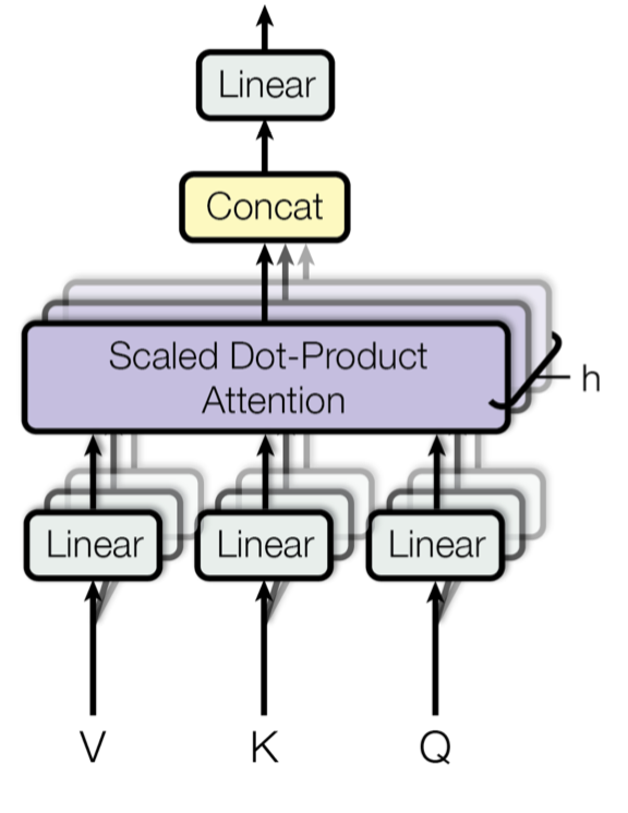
If single attention is like focusing with one lens, multi-head attention resembles the compound eye of an insect: multiple specialized perspectives combining to create a richer, more nuanced representation.
Each attention head learns to focus on different types of relationships:
MultiHead(Q, K, V) = Concat(head_1, ..., head_h)W^O
where head_i = Attention(QW_i^Q, KW_i^K, VW_i^V)
The projection matrices (W^Q, W^K, W^V) allow each head to develop its own “viewing angle” by transforming the input representations into different subspaces. One head might specialize in syntactic relationships (subject-verb connections), another in semantic associations (related concepts), and yet another in long-range dependencies (pronouns to their antecedents). This specialization emerges naturally through training, without explicit instruction. A beautiful example of self-organization in neural systems.
The final linear projection W^O combines these diverse perspectives into a unified representation, much like how your brain integrates information from different sensory modalities to create a coherent perception of reality.
Once the Transformer has identified what information is relevant, it needs to process and transform that information into something useful, much like how your digestive system breaks down food into nutrients your body can actually use.
The Feed-Forward Network: The Transformer’s Digestive System#
While attention mechanisms capture the spotlight in most Transformer discussions, the feed-forward networks (FFNs) quietly perform the heavy lifting of information processing.
These networks, positioned after each attention layer, serve as the Transformer’s metabolic engine, taking the relationally-enriched representations from attention and transforming them through nonlinear processing. The architecture is deceptively simple:
FFN(x) = max(0, xW₁ + b₁)W₂ + b₂
This represents a two-layer neural network with a ReLU activation function sandwiched between them. But don’t let the simplicity fool you, this component typically contains the majority of the Transformer’s parameters, making it the model’s primary repository of learned knowledge.
The Expansion and Compression Dance#
The feed-forward network follows a distinctive expand-then-compress pattern.
The first layer typically expands the representation to a much higher dimension (often 4x the model dimension), creating a rich, high-dimensional space where complex transformations can occur. Think of this as breaking down complex ideas into their constituent parts for detailed examination.
The ReLU activation introduces crucial nonlinearity, allowing the network to learn complex, non-trivial transformations. Without this nonlinearity, multiple linear layers would collapse into a single linear transformation, mathematically equivalent but computationally wasteful.
The second layer then compresses this expanded representation back to the original dimension, synthesizing the processed information into a form that can integrate with the rest of the architecture. This expansion-compression cycle resembles how we might explode a complex problem into detailed analysis before synthesizing our findings into actionable insights.
The Memory Bank of Knowledge#
Recent research suggests that feed-forward networks function as associative memories, storing factual knowledge and retrieving it based on input patterns. When you ask a language model “What is the capital of France?”, it’s likely the feed-forward layers that contain and retrieve the “Paris” association, triggered by the specific pattern of the query.
This perspective explains why larger models with more FFN parameters tend to know more facts, they simply have more storage capacity in their associative memory banks.
Just as a biological organism needs a circulatory system to maintain homeostasis and ensure nutrients reach every cell, the Transformer requires its own stabilizing infrastructure to enable deep, stable learning.
Layer Normalization and Residual Connections: The Transformer’s Circulatory System#
While attention and feed-forward networks capture most of the spotlight, two seemingly modest components quietly ensure the Transformer’s architectural stability: layer normalization and residual connections. These elements work in concert like a sophisticated circulatory system, maintaining the health of information flow throughout the network’s many layers.
Without these stabilizing mechanisms, training deep Transformers would be nearly impossible. Gradients would vanish or explode, representations would drift to extreme values, and the delicate balance between different components would collapse.
Residual Connections: The Information Highways#
Residual connections, borrowed from computer vision’s ResNet architecture, create “skip highways” that allow information to bypass processing layers entirely. In mathematical terms, instead of simply computing F(x), each sub-layer computes x + F(x), where x is the input and F(x) is the transformation performed by that layer.
This seemingly simple addition has profound implications. It ensures that even if a layer learns to contribute nothing (F(x) = 0), the input can still flow through unchanged. More importantly, during backpropagation, gradients can flow directly back through these skip connections, preventing the vanishing gradient problem that plagued earlier deep architectures.
Think of residual connections as express lanes on a highway system: while local traffic (the layer transformations) handles detailed processing, the main flow of information can always take the express route when needed.
Layer Normalization: The Homeostatic Regulator#
Layer normalization serves as the Transformer’s homeostatic mechanism, maintaining stable activation distributions across the network. Unlike batch normalization, which normalizes across the batch dimension, layer normalization operates across the feature dimension for each individual example:
LayerNorm(x) = γ × (x - μ) / σ + β
Where μ and σ are the mean and standard deviation computed across the feature dimension, while γ and β are learned scaling and shifting parameters.
This normalization prevents activation values from growing too large or too small, which could cause training instabilities or push the network into saturated regions where gradients become negligible. By keeping activations in a reasonable range, layer normalization enables the use of higher learning rates and more stable training dynamics.
The Synergistic Dance: Pre-Norm vs Post-Norm#
The original Transformer placed layer normalization after each sub-layer (post-norm), but many modern implementations use pre-normalization, applying it before each sub-layer. This architectural choice profoundly affects training dynamics:
Post-Norm Architecture:
x + LayerNorm(SubLayer(x))
Pre-Norm Architecture:
x + SubLayer(LayerNorm(x))
Pre-norm architectures tend to be more stable during training, as the normalization happens before potentially destabilizing transformations. However, post-norm can lead to better final performance, though it requires more careful tuning. This trade-off exemplifies how seemingly small architectural decisions can have cascading effects throughout the system.
The Gradient Flow Perspective#
Together, these components create what researchers call “gradient superhighways”, direct paths for gradient information to flow from the output back to early layers. Without residual connections, gradients would need to pass through every transformation, potentially vanishing to nothing. Without layer normalization, the scale of gradients could vary wildly between layers, making optimization unstable. The combination enables the training of models with hundreds of layers, something that would have been impossible with earlier architectures. It’s a beautiful example of how engineering solutions inspired by biological systems (homeostasis) and highway design (skip connections) can solve fundamental computational challenges.
Now that we’ve dissected the individual organs, let’s see how they work together in the two main architectural configurations that power modern AI.
Encoder-Decoder vs. Decoder-Only: Two Evolutionary Paths#
The original Transformer architecture featured both encoder and decoder stacks working in tandem, but the field has since evolved into two distinct evolutionary branches, each optimized for different computational philosophies and use cases.
The Encoder-Decoder Architecture: Comprehension Then Generation#
The encoder-decoder design embodies a “think first, then speak” approach to sequence processing. The encoder stack processes the entire input sequence in parallel, building increasingly sophisticated representations through its layers. Each encoder layer applies self-attention and feed-forward processing to understand relationships within the input, creating a rich contextual understanding.
The decoder operates differently, it generates output autoregressively while attending to both the encoded input representations (through cross-attention) and its own previously generated tokens (through masked self-attention). This cross-attention mechanism allows the decoder to selectively focus on relevant parts of the input when generating each new token.
This architecture excels at tasks requiring explicit input-output mapping: machine translation (“Translate this German text to English”), summarization (“Summarize this article”), and question answering (“Given this passage, answer the question”). Models like T5, BART, and early neural machine translation systems exemplify this approach.
The Decoder-Only Revolution: Unified Processing#
The decoder-only architecture represents a philosophical shift toward unified, autoregressive processing. Instead of separating comprehension and generation phases, these models treat everything (prompts, context, and generated responses) as a continuous sequence to be processed autoregressively. This simplification brings surprising benefits. GPT-style models demonstrate that the same autoregressive objective that generates text can also learn to understand, reason, and follow instructions. The decoder’s masked self-attention ensures that information flows only from previous positions to future ones, maintaining the causal structure necessary for language generation while enabling rich contextual understanding. Modern large language models like GPT-4 and Claude have proven that decoder-only architectures can achieve remarkable versatility, handling tasks from creative writing to mathematical reasoning to code generation, all through the same autoregressive framework.
Autoregressive Inference: The Art of Sequential Prediction#
Understanding how modern language models generate text reveals the fascinating dance between mathematical precision and emergent intelligence. Let’s trace through exactly what happens when you interact with an instruction-tuned model, keeping in mind that we’re simplifying the actual process to illustrate the underlying mechanisms.
The Generation Process: A Step-by-Step Journey#
Imagine you’ve just typed: “The weather in Paris today is”.
Imagine you’ve asked an instruction-tuned model: “Explain why the sky appears blue.” Here’s a simplified version of what unfolds inside the Transformer (note that actual tokenization and processing is more complex, but this illustrates the core principles):
Step 1: Initial Processing Your question gets tokenized, let’s say into tokens representing: [“Explain”, “why”, “the”, “sky”, “appears”, “blue”, “.”]. Each token receives its embedding and positional encoding. The model also processes this within the context of its instruction-following training, recognizing this as a request for an explanation.
Step 2: Parallel Context Building All tokens flow through the Transformer’s layers simultaneously. Attention mechanisms activate: “Explain” signals that a pedagogical response is needed, “sky” and “blue” connect to scientific knowledge about light scattering, and the question structure indicates the model should provide a clear, educational answer rather than simply continue the text.
Step 3: The First Prediction At the position where generation begins, the model outputs a probability distribution. For an instruction-tuned model, this might heavily favor tokens that start explanatory responses: “The” (0.25), “Light” (0.15), “When” (0.12), “This” (0.08), very different from what a base model trained only on next-token prediction might generate.
Step 4: Selection and Continuation Let’s say “The” gets selected. The sequence in the model’s context now includes your question plus: “The”. The model continues, perhaps selecting “sky” next, then “appears,” building toward: “The sky appears blue because…”
Step 5: The Autoregressive Loop Each new token shifts the context and influences the next prediction. When the model reaches “because,” the attention mechanism now focuses heavily on the scientific explanation it needs to provide. The feed-forward networks retrieve knowledge about Rayleigh scattering, wavelength properties, and atmospheric physics.
Key Generation Parameters#
Several crucial parameters control how this anatomical process unfolds during generation. Let’s see some of them:
Temperature (τ): Controls the “sharpness” of the probability distribution by scaling the logits before applying softmax:
P(token) = softmax(logits, τ). Temperature ranges from 0 to 1 in most frameworks. Lower temperature (approaching 0) makes the model more confident and deterministic, while higher temperature (approaching 1) increases randomness and creativity. At temperature 0, the model always selects the highest probability token.
Top-k Filtering: Restricts sampling to only the k most probable tokens, effectively “amputating” the long tail of unlikely possibilities and focusing the model’s attention mechanism on the most relevant options.
Top-p Sampling: Dynamically selects tokens whose cumulative probability mass reaches p, adapting the selection pool based on the model’s confidence distribution.
Maximum Length: Determines when the autoregressive process terminates, preventing infinite generation loops.
The Mechanical Reality#
What makes this process remarkable is its mechanical simplicity. Each forward pass is identical: embeddings flow through attention layers, get processed by feed-forward networks, pass through normalization and residual connections, and produce a probability distribution. Yet this repetitive mechanical process, guided by the parameters above (and many more), creates the appearance of reasoning, creativity, and understanding. The Transformer’s anatomy enables this autoregressive dance: positional encoding maintains sequence awareness, attention mechanisms preserve context relationships, feed-forward networks contribute learned knowledge, and the stabilizing components ensure consistent processing throughout the generation loop.
Conclusion: The Computational Body Revealed#
Our anatomical journey through the Transformer has revealed an architecture of remarkable elegance and mechanical precision. Like dissecting a biological organism, we’ve traced how each component serves a vital function in the emergence of intelligent behavior. The positional encoding provides spatial awareness in a parallel processing world, attention mechanisms create selective focus and relational understanding, feed-forward networks store and retrieve vast knowledge, and layer normalization with residual connections maintain the stability necessary for deep computation. When these components work together through the autoregressive generation process, mathematical operations transform into behavior that appears genuinely intelligent.
Perhaps the most profound insight from our dissection is how relatively simple mathematical operations (matrix multiplications, dot products, nonlinear transformations) can combine through careful architectural design to produce such sophisticated capabilities. The Transformer doesn’t think as humans do, but through the orchestrated interaction of its anatomical components, it achieves something functionally remarkable. Understanding this anatomy provides the foundation for future innovations. Whether improving attention efficiency, enhancing knowledge storage in feed-forward layers, or developing new normalization techniques, progress requires deep appreciation of how each organ contributes to the computational whole. The Transformer has already reshaped our technological landscape, but our anatomical exploration suggests we’ve only begun to understand what’s possible when we truly comprehend the mechanics of artificial intelligence. Like early anatomists whose detailed observations enabled medical breakthroughs, understanding the Transformer’s internal structure opens pathways to even more capable architectures. In the end, the Transformer stands as a testament to the power of thoughtful design; proof that complex intelligence can emerge from the careful orchestration of simple, well-understood components.