NOTE: This post was written before the Machine Learning Surgeon got in charge of the blog, that’s why there are no references to surgical operations!
Large Language Model. How many times did you read that term? Nowadays, the popularity of Artificial Intelligence is to be attributed to the exceptional results obtained, in the past few years, by applications that leverage large models. Surely, you know the most popular one, ChatGPT, made by OpenAI.
When I first started learning about neural networks -about 5 years ago-, one of the key questions I had was if it would be possible to know, a priori, the minimum number of parameters that a network must implement to achieve a certain metric value when solving a specific problem. Unfortunately, as far as I know, there is no such theorem. Surely, we know about convergence theorems -like the Universal Approximation Theorem-, but nothing tells us the optimal number of parameters, given an architecture and a problem to solve.
A very interesting methodology is the Cascade Correlation, which is a constructive approach for obtaining a network that solves a specific problem. However, this methodology is impractical in modern times: the size of neural networks is just too big, especially when talking about LLMs, which typically span from 7 to 70 billion parameters.
Therefore, a follow-up question: given a trained, large network, can we reduce its size while maintaining the same accuracy?
That’s the key idea behind Pruning.
Pruning for Sparsity#
Let’s start from a biological point of view: humans drastically reduce the number of synapses per neuron from early childhood to adolescence. This has been shown in various papers (e.g. Synapse elimination accompanies functional plasticity in hippocampal neurons) and it is a way for the brain to optimize its knowledge and remove redundancy. As often happens, this concept can also be applied to learning architectures.
Assume to have a relatively large neural network that has been trained to approximate the solving function for a given problem, which was described by a dataset. This means that, by training, we minimized the loss function defined as:
\(\mathrm{L}(\theta, \mathcal{D}) = \frac{1}{N}\sum_{(x,y)\in(X,Y)}{L(\theta, x, y)}\)
where \(\theta\) represents the weights of the network and \(\mathcal{D}\) symbolizes the data used to train it.
Let’s now assume that we are capable of pruning the weights \(\theta\), therefore obtaining \(\theta_{pruned}\). Our objective is to get approximately the same loss value when using the pruned weights. In math:
The advantage here is obvious: \(\theta_{pruned}\) is a smaller, more efficient model that is capable of replicating the accuracy of a bigger, slower model.
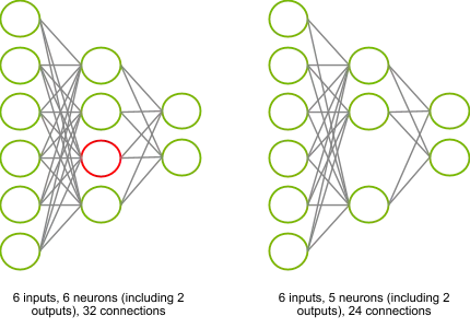
Take a look at the picture below: by pruning the red neuron, we remove 8 connections and the activation of the neuron itself. If both the networks had the same accuracy, we would prefer the right one, because its inference is more efficient.
Choosing what to prune#
The pruning criterion is a very important factor to take into account, and research is still very active in this specific field. The common idea that unites all the pruning criteria is to prune parameters that are less useful in solving the problem. Therefore, we need a metric that describes the importance of a neuron in the overall network.
In this post, I’ll only talk about the Magnitude-based criterion, but I encourage interested readers to research other methodologies, e.g. Scaling-based pruning, Regression-based pruning, and Percentage-of-zero-based pruning.
The Magnitude-based criterion selects parameters to prune based on, guess what, their magnitude, therefore using an L_p norm. For example, we could choose to use an L_1 norm (a.k.a. the absolute value) as the importance metric for the parameter:
\(importance(\theta_{i}) = ||\theta_{i}||\)
The rationale behind this is that the smaller the parameter, the less its influence is in the activation of the neuron.
So, if you assume to have a neural network with 100 parameters, and you want to prune 80% of them, you should first define an importance metric, then compute it for each parameter, sort the result, and pick the top-k parameters for that importance.
Pruning Granularity#
Another key concept for pruning is granularity. We can proceed either by selecting parameters in an unstructured way or using a pattern. Let’s just see two examples to grasp this concept.
Assume to have a matrix that represents the parameters we want to prune:
\(\mathsf{P} \in \mathcal{R}^{m,n} \)
and also assume that we picked the L_2norm as the importance metric for the Magnitude-based criterion.
Then, we can perform either:
unstructured pruning: we iterate over each parameter, compute its L_2 norm, and prune it if it’s not in the top-k percentage of neurons per importance.
structured pruning: instead of computing the L_2 norm for the single parameter, we first select a pattern. Let’s keep things simple and assume that our pattern corresponds to the row of the matrix P. Therefore, we will not prune the single parameter, but instead, we will prune the rows that do not belong to the top-k percentage of the highest-importance rows in the matrix.
The picture below depicts the difference between the two approaches.
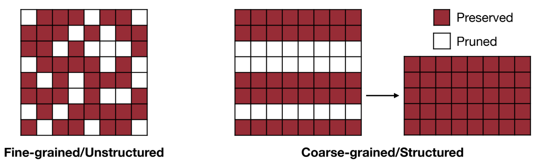
This picture also foretells the advantages of pattern-based pruning, which I will explain in a later section.
Pruning Ratio#
The pruning ratio is the last key concept we need to understand. Luckily for us, it’s quite straightforward. The ratio indicates how much sparsity we want in our neural network.
For example, if we pick a uniform pruning ratio of 80%, we will remove 80% of the parameters of the network, which will be selected based on the criterion and importance measure, defined before.
The word “uniform” is not randomly put. In fact, we can also provide a different pruning ratio for different levels of the network architecture. For example, we could select different pruning ratios for different layers of the architecture, or different channels.
There are several methodologies to find the optimal pruning ratio, but I will not cover them in this introduction.
Does pruning work?#
Yes, and incredibly, if done correctly.
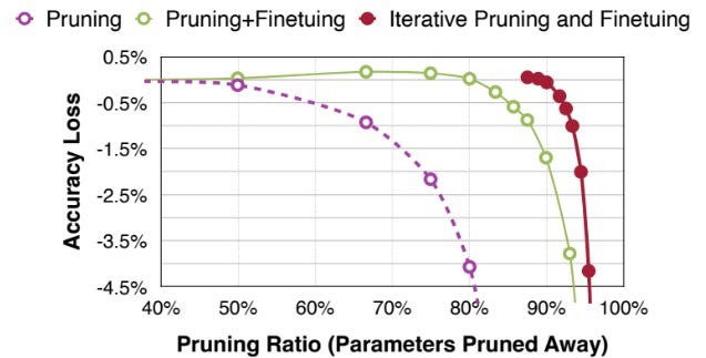
The first thing to notice is that we should always retrain the network after pruning. This is done because, when pruning aggressively (typically > 90%), the accuracy of the network drops significantly. Performing a fine-tuning step is crucial to retain information in the parameters that survived the pruning phase, and therefore stabilize the accuracy of the model.
This excellent picture from efficientml.ai very clearly depicts this concept
Computations with sparsity#
When talking about the pruning granularity, we saw the conceptual difference between unstructured and structured pruning. Let’s consider again the matrix:
\(\mathsf{P} \in \mathcal{R}^{m,n}\)
Let’s now assume another matrix, which will be multiplied with matrix \(\mathcal{P}\):
\(\mathsf{L} \in \mathcal{R}^{n,l}\)
Computing \(\mathsf{P}\) x \(\mathsf{L}\) in the most straightforward way possible, we perform a number of MACs equal to:
\(MACs = m \times n \times l\)
If we manage to reduce the number of rows of \(\mathsf{P}\) -therefore reducing \(m\)-, it’s easy to see how the number of computations is reduced, as the size of the matrix \(\mathsf{P}\) itself.
In the unstructured case, instead, we did not shrink the dimension of the \(\mathsf{P}\) matrix, but we just made it sparse, by setting some elements to 0. How are we getting a benefit from that?
That’s the catch: we don’t. If we don’t have the availability of an efficient system for sparsity, we will not get any benefit from having a sparse \(\mathsf{P}\) matrix. This applies to both the computational and memory point of view.
The topic of efficient systems for sparsity computations is just too vast to be discussed here. Let me know if you are interested in the topic and would like to read a post that delves into it!
Conclusions#
In this brief introduction to pruning for efficient neural networks’ inference, we learned about the three key concepts for this methodology: selecting the parameters to prune, the pruning granularity, and the pruning ratio.
We also saw how much benefit can be obtained by pruning a model, both in terms of computational and memory complexity.
There’s still much to say about this technique, so the learning doesn’t stop here! I hope this post was a good introduction, and that it conveyed well to you these basic concepts.