During the first year of my Master’s Degree in Computer Science, I had to complete a project for a Machine Learning course. It involved implementing a small feed-forward neural network framework from scratch, using only numerical libraries and coding elements such as loss functions, backpropagation, and the feed-forward step.
That project was crucial for me because it revealed an inconvenient truth: matrix multiplication is the most fundamental aspect of Machine Learning. Hence, I named my project “ML is ML”: Machine Learning is Matrix Multiplication. Although the course professor didn’t fully appreciate the title, it still earned me the highest grade. Because deep down, they knew it was true. It was, indeed, an inconvenient truth.
NOTE: Yes, I’m well aware that tensor contraction is not the same as matrix multiplication. Still, the “ML is ML” joke only works when talking about matrices, so stick with it.
However, this is not the place to explain why matrix multiplication is so fundamental to modern AI. Besides, if you’re reading this blog, you probably already know.
Instead, as Machine Learning Surgeons, we should ask ourselves how such an important operation is implemented to fully utilize the power of GPUs. It’s easy to implement something, but it’s much harder to make it run fast! Just like humans need to train their reaction times to do tasks like driving an F1 car, we Machine Learning Surgeons must operate on the muscle fibres of kernels in order to make them fast and powerful!
So, put on your gloves, wield your scalpels and let’s start the operation!
The First Cut#
Since you’re still a pratictioner, I’ll walk you through the simplest matrix multiplication kernel. But first, there is a basic concept that you have to grasp before proceeding with the code.
Matrix Linearization#
As you may have learned from the Hello CUDA article, when writing CUDA kernels, we typically use block and thread indices to select elements for computation. But what happens when dealing with higher-dimensional data structures, such as matrices? Moreover, how is memory organized on GPUs when dealing with such data structures?
In CUDA, memory on the device is managed linearly, meaning it is stored as a single, contiguous block of memory. Therefore, matrices are stored in this contiguous block of memory in a row-major order. Linearization involves mapping the multi-dimensional indices of a matrix to a single-dimensional index. It’s much easier to do than to explain.
Consider a matrix \(\mathrm{A} \in \mathrm{R}^{\mathrm{N} x \mathrm{N}}\) stored in a row-major order, which is the representation used by CUDA. The linear index of the element \(\mathrm{A}_{i, j}\) (i-th row and j-th column of \(\mathrm{A}\)) is simply given by \(i * \mathrm{N} + j\). This is because in the row-major representation, the array that represents the 2D matrix is a continuous sequence of the rows of the matrix. Therefore, to acces the item \(\mathrm{A}_{i, j}\) we must skip \(i\) rows, doing \(i * \mathrm{N}\) and sum to it the column index \(j\).
This is a fundamental concept to understand before proceeding, as we will be performing numerous memory accesses using this technique.
A Naive Kernel#
Great! Now you are ready to fully understand the simplest matrix multiplication kernel. Keep in mind that I’ll avoid writing all the usual boilerplate code for instantiating variables on the host, moving data to the device, and printing results. If you have any doubts, you can check the full code here
| |
You should be able to understand most of this code, but let’s quickly walk through it.
In lines 2-3, we define the index of the row and column of the matrix element that the thread will use for the dot product computation. Remember that the mathematical notation and the CUDA representation are inverted. While in mathematical notation we use the x-axis for referring to the rows and the y-axis for referring to the columns, in CUDA we use the y-components to compute the row index and the x-components to compute the column index.
Line 5 simply checks the index boundaries. We must check this condition because we will likely spawn more threads than there are elements in the matrix, so some threads may compute out-of-bounds indices.
Lines 6-10 perform the actual dot product computation. We start by initializing a local variable to accumulate the result. Given that this is a local scalar variable, it will be stored in a register, the fastest type of memory available. This approach works well because the dot product, which involves summing the products of corresponding elements, can be computed incrementally. Remember this, as it will be essential for the upcoming optimization steps!
Line 7 defines the loop that allows the thread to iterate over all elements of the rows of A and the columns of B. In each iteration, we accumulate the value by adding the product of the linearized row element from A and the linearized column element from B. If you find it difficult to visualize the linearizations, I suggest writing out a few loop iterations on a piece of paper.
Lastly, line 10 stores the computed dot product into the linearized element of C.
For completeness, I will also include the kernel invocation. Keep in mind that you can use the ceil() function for the gridSize
dim3 blockSize(16, 16);
dim3 gridSize((N + blockSize.x - 1) / blockSize.x, (N + blockSize.y - 1) / blockSize.y);
matMulKernel<<<gridSize, blockSize>>>(d_C, d_A, d_B, N);
Advanced Surgical Techniques#
Now that we have a basic implementation, let’s pause to consider the kernel’s behavior.
A subtle issue to notice is that all memory accesses we perform are done using Global Memory. If you need an explanation about memory types in CUDA, please read this blog post. In brief, Global Memory is much slower compared to other types of memory, such as Shared Memory. As a result, we are wasting time with these accesses.
Furthermore, the kernel is actually performing more data loads than necessary. Consider the first thread of the grid, let’s call it \(thread_{0,0}\). This thread will compute the indexes \((0,0)\), therefore it will load the elements \(\mathrm{A}_{0,0}\) and \(\mathrm{B}_{0,0}\) in its first iteration. Then, given that we perform a loop over the elements of the matrices, \(thread_{0,0}\) will also load \(\mathrm{A}_{0,1}\) and \(\mathrm{B}_{1,0}\), \(\mathrm{A}_{0,2}\) and \(\mathrm{B}_{2,0}\) and so on.
Let’s now consider the second thread of the grid which we will call \(thread_{0,1}\). This kernel will load \(\mathrm{A}_{0,0}\) and \(\mathrm{B}_{0,1}\), then \(\mathrm{A}_{0,1}\) and \(\mathrm{B}_{1,1}\), then \(\mathrm{A}_{0,2}\) and \(\mathrm{B}_{2,1}\) and so on.
Notice how element \(\mathrm{A}_{0,0}\) is loaded by both kernels. Since Global Memory access is not shared between threads, each thread must perform a separate loading operation to obtain the value of the matrix element. In fact, in this example, it is easy to see how all elements of \(\mathrm{A}\) are loaded by both kernels. I encourage you to continue this analysis on your own so that you can see for yourself that the same is true for all elements of \(\mathrm{B}\) as well.
It’s now clear what we can do to optimize this kernel: use Shared Memory to improve the speed of loading operations, while also avoiding redundant loading operations within a block. Specifically, we will use tiling to manage the memory traffic reduction factor. If we assume 16x16 tiles, we can reduce the memory traffic by a factor of 1/16 compared to the naive implementation, because all threads will cooperate for the memory accesses. In general, given a tile size \(T_N\), we reduce the memory traffic by \(1/T_N\). If we take this idea to the extreme, by setting \(N = T_N\)we could load the entire matrix into a single tile in Shared Memory, thereby maximizing the reduction in memory traffic. However, this is rarely feasible. In real-world scenarios, the size of matrices is usually so large that the entire matrix cannot fit into the Shared Memory.
Understanding the balance between tile size and Shared Memory usage is crucial for optimizing performance. While larger tiles can reduce memory traffic, they are limited by the available shared memory, and practical implementations must account for this constraint.
Advanced Incision Techniques: Tiling#
NOTE: A bit of linear algebra ahead, proceed with caution.
As mentioned before, the dot product can be computed incrementally. We can leverage this property to split the computation of a single dot product into phases, which correspond directly to tiles. Let’s consider two matrices \(\mathrm{A} \in \mathrm{R}^{16x16}\) and \(\mathrm{B} \in \mathrm{R}^{16x16}\). We want to perform a matrix multiplication which result will be represented by \(\mathrm{C} \in \mathrm{R}^{16x16}\).
Let’s split \(\mathrm{A}\) and \(\mathrm{B}\) into 4 tiles of size 4x4 each, let’s call them \(\mathrm{T_A}_{i,j} \in \mathrm{R}^{4x4}, i = 0, 1, 2, 3 \land j=0,1,2,3\) and \(\mathrm{T_B}_{i} \in \mathrm{R}^{4x4}, i = 0, 1, 2, 3 \land j=0,1,2,3\).
Assume we want to compute the first element \(\mathrm{C}_{0,0}\). In the previous kernel code, we fully loaded the first row of \(\mathrm{A}\) and the first column of \(\mathrm{B}\) and performed the dot product. Now, instead, we will use tiles.
Since the dot product can be computed incrementally, we can procede as follows:
Load two tiles into memory. We load tiles based on the current phase. At the start, we are in phase 0, so we load \(\mathrm{T_A}_{0}\) and \(\mathrm{T_B}_{0}\).
Compute all elements of the dot product that can be computed with the loaded tiles. Note that these are partial computations! The remaining parts of the computations will be performed in subsequent phases. In phase 0, we would compute:
- \(\mathrm{C}^{0}_{0,0} = \sum_{k=0}^{3} \mathrm{T_A}_{0,k} * \mathrm{T_B}_{k,0}\)
- \(\mathrm{C}^{0}_{0,1} = \sum_{k=0}^{3} \mathrm{T_A}_{0,k} * \mathrm{T_B}_{k,1}\)
- \(\mathrm{C}^{0}_{1,0} = \sum_{k=0}^{3} \mathrm{T_A}_{1,k} * \mathrm{T_B}_{k,0}\)
- \(\mathrm{C}^{0}_{1,1} = \sum_{k=0}^{3} \mathrm{T_A}_{1,k} * \mathrm{T_B}_{k,1}\)
Notice that the notation \(\mathrm{C}^{0}\) indicates the computation of and element of \(\mathrm{C}\) for the first phase, phase 0. Subsequent phases will sum upon this initial computation to obtain the final result.
Then, increase the phase counter and repeat the process until all computational phases are complete. Note that the number of phases is \(N/size\_of\_tile\), where \(N\) is the dimension of the square input matrices.
After all the computations for a point of \(\mathrm{C}\) are done, store the result in the actual output matrix.
If you’ve made it through this notation hell, you’re ready to see the actual kernel code!
Brain Cells Cooperating#
An attentive reader might ask: How is this algorithm faster? From a mathematical and algorithmic perspective, the benefits of splitting computations and using tiling might not be immediately clear and can even seem to complicate matters. However, tiling is crucial for optimizing memory access patterns, as we discussed earlier. Let’s examine the code to understand how tiling enhances performance in practice:
| |
In lines 2-3, we define the two data structures used to load the tiles from
\(\mathrm{A}\) and
\(\mathrm{B}\). We use the __shared__ keyword to specify that this memory allocation will be performed in Shared Memory.
In lines 5-8, we define some variables to store the block and thread IDs for both the x and y dimensions. This is done for convenience, as writing these values explicitly each time would make the code less readable. Since we are not even close to register saturation, it’s a luxury we can afford. In lines 10-11, we simply compute the row and column indexes, since the kernel assumes that each thread will compute one element of \(\mathrm{C}\).
Line 15 starts the for loop that iterates over the computational phases. As mentioned before, there are \(N/size\_of\_tile\) phases in total. For simplicity, we assume that the dimension of the matrices is divisible by the tile size, so the division yields a whole number.
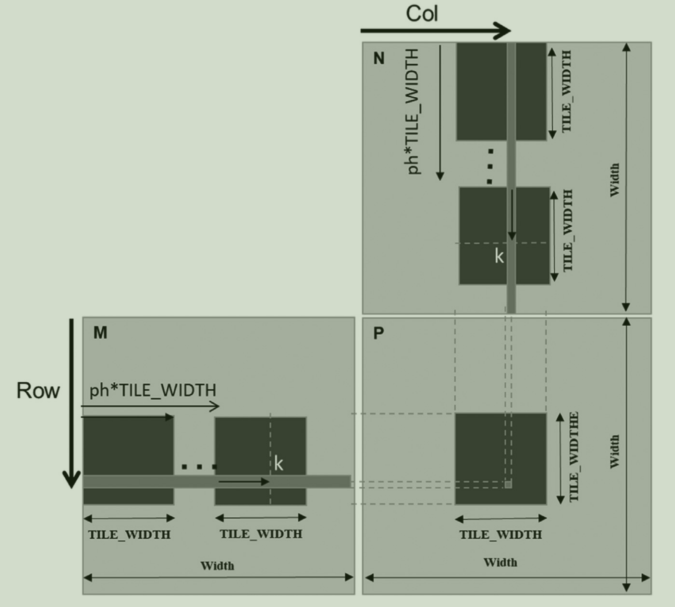
Finally, lines 16-18 demonstrate thread cooperation. Here, the threads use the shared variables Ads and Bds to load the elements into the tiles for the current phase, ph. If you look closely at the index computations, you’ll see they are almost identical to those used in the naive implementation. The key difference is that here we skip elements by using the contribution ph * TILE_WIDTH. This adjustment is necessary because, at each phase, we have already performed the required computations using elements from the previous phases (and therefore the previous tiles). The picture below illustrates this behavior perfectly.
Furthermore, line 18 introduces a barrier synchronization. Since threads are loading elements into memory asynchronously, we must ensure that all elements of the tiles for the current phase have been loaded before proceeding with the computation of the partial dot product.
Lines 20-22 perform exactly the operation listed as step 2 in the previous section, which is the computation of the partial dot product using the previously loaded tiled elements. This step also requires a barrier synchronization, as the elements stored in Ads and Bds will be overwritten in the next phase. We must ensure that all threads have finished the computation of the partial dot product for the current phase before proceeding to the next phase.
Finally, in line 26, we write the computed value to the output matrix C.
Flexible Incisions: Arbitrary Tile Size#
In our previous kernel code, we assumed that the matrix size is divisible by the tile size. However, this is a strong assumption that may not always hold true. Is there a way to relax this assumption? Yes, through boundary checking.
First, let’s examine what happens when the matrix size is not divisible by the tile size.
The first observation we make is that issues arise only with the last tile. For instance, consider a matrix \(\mathrm{A} \in \mathrm{R}^{16,16}\) and tiles \(\mathrm{T_A}_{i,j} \in \mathrm{R}^{3x3}, i = 0,1,2,3,4,5 \land j=0,1,2,3,4,5\). For example, the tile \(\mathrm{T_A}_{0,0}\) is within the bounds of the matrix, so it does not present any issues. However, a tile like \(\mathrm{T_A}_{5,5}\) is problematic because it extends beyond the matrix boundaries. This issue occurs because 16 is not divisible by 6, therefore some tiles will go out of bounds.
What exactly happens when we go out of bounds? If we access an element beyond the last row, we will end up accessing elements from subsequent rows due to the row-major linearization of the matrix. This will lead to incorrect results. When it comes to columns, accessing elements outside the allocated memory of the matrix can have various outcomes. We might load random values, load zeros, or even cause a kernel crash, depending on the system and its handling of such memory accesses.
We cannot solve this problem by simply not using the aforementioned tiles, as this would leave some elements unprocessed.
To address this, we can perform boundary checks to ensure that the computed x and y indexes for the thread are responsible for loading valid elements. The same checks apply to the output indexes. For rows, we check that \(row \text{\textless} Width \land (ph * TILE\_WIDTH) \text{\textless} Width\). For columns we check that \((ph * TILE\_WIDTH + ty) \text{\textless} Width \land Col \text{\textless} Width\). If these conditions are not met, we load a neutral value, such as 0.0, into shared memory for the operation, so that such elements will not effect the computations.
Lastly, we will store the value only if both the row and column indexes are within the bounds of the output matrix. Therefore, the kernel code is modified as follows:
__global__ void matMulKernel(float* A, float* B, float* C, int Width) {
    __shared__ float Ads[TILE_WIDTH][TILE_WIDTH];
    __shared__ float Bds[TILE_WIDTH][TILE_WIDTH];

    int bx = blockIdx.x;
    int by = blockIdx.y;
    int tx = threadIdx.x;
    int ty = threadIdx.y;

    int row = by * TILE_WIDTH + ty;
    int col = bx * TILE_WIDTH + tx;

    float Cvalue = 0;

    for(int ph = 0; ph < ceil(Width/float(TILE_WIDTH)); ++ph) {
        if(row < Width && ph * TILE_WIDTH + tx < Width)
            Ads[ty][tx] = A[row * Width + ph * TILE_WIDTH + tx];
        else
            Ads[ty][tx] = 0;
        if (ph * TILE_WIDTH + ty < Width && col < Width)
            Bds[ty][tx] = B[(ph * TILE_WIDTH + ty) * Width + col];
        else
            Bds[ty][tx] = 0;
        __syncthreads();

        for(int i = 0; i < TILE_WIDTH; ++i) {
            Cvalue += Ads[ty][i] * Bds[i][tx];
        }
        __syncthreads();
    }

    if (row < Width && col < Width)
        C[row * Width + col] = Cvalue;
}
Closing the Incision#
We’ve come a long way in our exploration of matrix multiplication in CUDA, haven’t we? We began with the basics—our “first cut”—where we learned how to implement a straightforward matrix multiplication kernel. From there, we moved on to the exciting phase of optimization and refinement, focusing on making our GPU computations faster and more efficient. By leveraging shared memory with tiling, we achieved significant performance improvements. We also incorporated boundary checking to allow for flexible tile sizes.
Fun fact: adapting the boundary-checked, tiled version of the kernel to support rectangular matrices is surprisingly straightforward! Just follow these steps:
- Replace
Widthwith unsigned integer arguments:j,k,l. - Update
Widthfor Matrix Heights and Widths:- Replace
Widthwithjwhere it refers to the height of matrixAor the height of matrixC. - Replace
Widthwithkwhere it refers to the width of matrixAor the height of matrixB. - Replace
Widthwithlwhere it refers to the width of matrixBor the width of matrixC.
- Replace
That’s it, you just wrote a general matrix multiplication CUDA kernel!
What? You’re not convinced? You don’t trust your brilliant doctor?!
I see that you want proof. You want some empirical data that proves that the optimizations we saw today actually worked! Fear not! In the next blog post, we’ll dive into the art of profiling CUDA kernels. I’ll guide you through the process of using tools like NVIDIA’s Nsight Compute to measure performance improvements, analyze memory usage, and make data-driven decisions about further optimizations. We’ll get down to the nitty-gritty details of profiling, so you can see exactly how your changes impact performance. It’s going to be a thrilling ride through the land of performance metrics and profiling!
Until then, happy coding, and remember to wash your hands!